Multiple Testing Method with Empirical Null Distribution in Leukemia Studies

By Raymond Wang and Jacob Benson

Introduction

Multiple testing analysis is a commonly used statistical practice in genetic research, often used to separate significant genes from a large pool of candidates. For example, in genome-wide association studies (GWAS), the multiple testing approach can be used to identify particular genes responsible for a certain disease. This is achieved through simultaneously conducting a large number of hypothesis tests between the control and experimental groups on each individual gene. With each hypothesis test’s t-statistics recorded, we can search through the data for anomalies and identify genes that might be correlated with the disease of our interest.

Acute Lymphocytic Leukemia (ALL) and Acute Myelogenous Leukemia (AML) are two common types of leukemia. According to the Children’s Hospital of Pittsburgh, ALL acounts for about 75 percent of childhood leukemia. It affects the growth of lymphocytes, a type of white blood cells that is normally responsible for one’s immunity, causing it to overproduce and crowding out other types of blood cells. On the other hand, AML causes the overproduction of granulocytes, another type of white blood cells. Identifying genes responsible for each of the two types of leukemia helps us to better understand their pathology as well as allows build statistical models adaptable for future studies and applications.

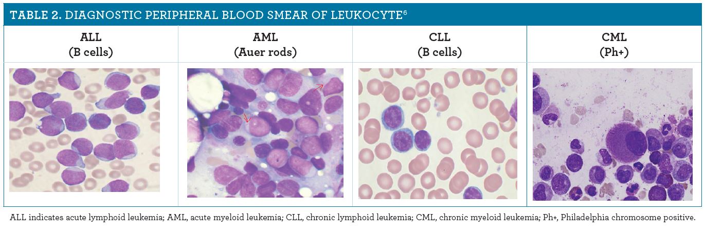
Sample images of AML, ALL, and other types of leukemia

In our study, we will apply a multiple testing model to a leukemia gene dataset to identify genes that are expressed differently between the two groups of leukemia. We will use both a theoretical null distribution and an empirical null distribution and compare and contrast the results between the two. We hypothesize that the empirical null distribution will yield more meaningful result than the theoretical null distribution.

Exploratory Data Analysis

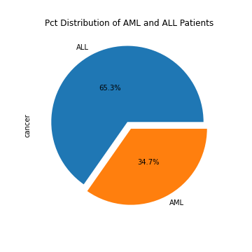
The dataset we will be using is collected by Harvard Professor of Pediatric, Todd Golub. It contains the gene expressions of 47 AML patients and 25 ALL patients. It is seperated into a training set and a test set. We will use these genetic data to perform pairwise t-tests between the ALL patients and the AML patients for every single gene. We will then transform the resulting t-statistics into standardized z-scores and apply quantile transformation.

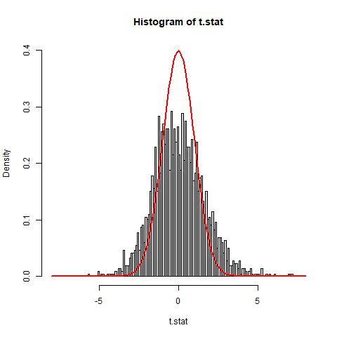
The histogram of the t-statistics show that the histogram of our data does not match well with the theoretical null distribution N(0,1) (solid red line). It appears that the histogram is both wider and shorter than the theoretical null. Furthermore, the data appears to have a slight right skew. To address this issue, we will use the estimation of parameter p₀ and an empirical estimation of the null distribution to address the additional variance.

Theory and Methods

Quantile Transformation

After some exploratory data analysis on the leukemia dataset, we discovered that the two groups, patients with AML and patients with ALL, have different variances across the dataset. This appears to be an issue for our hypothesis testing procedure, as the t-test function in R applies Welch’s t-test using approximation to the degrees of freedom in case of unequal variances between two groups. Since the degrees of freedom varies among samples, we must apply a quantile transformation on the t-statistics in order to obtain uniform distribution across our data.

To do this we found the tail areas (or probabilities) of each t statistic and their respective z scores in a normal distribution. Then we used the qnorm function to get the corresponding z scores for each area. The qnorm function takes the lower-tailed area and returns the corresponding z-value. After we input our areas we are now left with a normal distribution of z-scores that will allow us to use the empirical null distribution

Empirical Null Estimaton

We will estimate the empirical null distribution by estimating the fraction of true negatives. To do so, we separate the data into two sets, S₀ and S_A, where S₀ denotes all true negatives and S_A denotes all true positives. In our dataset, S₀ represents all genes that are uncorrelated with differentiating AML from ALL while S_A represents those genes that correlate. Furthermore, we define f₀(t) and f_A(t) to be the probability distribution of S₀ and S_A respectively. We will estimate the fraction p₀ of the number of true negatives over the number of samples so that the data distribution:

f(t) = p₀f₀(t) + (1-p₀)f_A(t)

is close to the the scaled density, p₀f₀(t) within an interval l₀ around the null distribution mean, 𝝁₀.

Notably, Efron et al. (2001) discusses that such application of the empirical null distribution must reach the following two requirements:

1. The number of tests, N, must be large.
2. A large majority of the tests must be within the null set, S₀.

False Discovery Rate Estimation

We will use false discovery rate (FDR) as our threshold metric for the statistical parametric map. The false discovery rate is defined as the rate of type I errors, the ratio between the number of false positives and the number of predicted positives. For our study, we set the level of threshold as u and define FP(u) and TP(u) to be the number of false positives and the number of true positives respectively under the threshold u. We will compute the false discovery rate under threshold u as the following:

FDR(u) = E[FP(u)/FP(u) + TP(u)]

We aim to control the threshold u to lower the false discovery rate. Notably, when u is large, we have fewer number of false positives, leading to a lowered FDR; however, increasing the threshold u also leads to increased false negatives. Ideally, we want to achieve a set FDR with the minimum level of threshold, u. To do this, we will first set a significance level ɑ for the FDR and then calculate the FDR for different levels of u and select the minimum u that satisfies the significance level of FDR. To put this in formula, we want to calculate

min_uFDR(u)

Compared to other thresholding criteria such as the family-wise error rate (FWER), which controls the rate of false positives among all samples, the FDR only controls the rate of false positives among the positives and therefore is more permissive of false positives by definition (Schwartzman et al., 2009). Since our goal is to identify the genes correlated with differentiating the AML from ALL, FDR is preferable as it allows some false positives as long as there are way more true positives.

Data Example

Using the quantile transformation method mentioned above, we obtain transformed z-scores from the t-statistics. From the graph below we see that the histogram still does not match well with the theoretical null (red dotted line) as it is much wider and shorter than the the theoretical null. We then estimate the parameter p₀ using the method mentioned in the secion above about empirical null estimation and compute that p₀ is approximately 0.595 for the theoretical null distirbution. This suggests that about 40.5% of the genes are expressed differently in the two types of leukemia patients from our data. The result is also observed from the scaled theoretical null distribution, which is plotted as the dashed red line, as it matches the histogram better than the theoretical null before the scaling but still does not solve the issue with the additional variances.

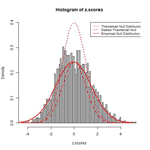
To solve this problem, we introduce an approach to estimate the empirical null distirbution using the median and an estimation of the standard deviation using the interquartile range (IQR). The estimation gives results p₀=0.933, μ=-0.066, and σ=1.534. The resulting distribution, observed as the red solid line in the graph above, provides a much better fit of the data than both the theoretical and scaled theoretical null distribution. the new estimated p₀ is much higher than the p₀ of the theoretical null, suggesting that only around 6.7% of the total genes are expressed differently between the two groups of patients. Since the empirical null distribution adjusts to the histogram’s additional variance due to confounding factors, we believe it will provide more realistic results and estimations of error rates.

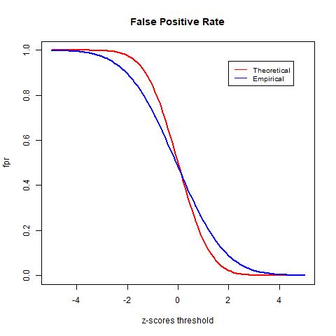
To test the accuracy of different null distributions, we will look at metrics such as the true positive rate (TPR), the false positive rate (FPR), and the false discovery rate (FDR). The TPR is calculated as the rate between the number of true positives (TP) and the number of true positives plus the number of false negatives (FN). It indicates the likelihood that an actual positive sample produces a positive testing result. The FPR is calculated as the rate between the number of false positives (FP) and the number of false positives and true negatives (TN). It indicates the likelihood of false positives. Lastly, the FDR is computed in equation (2) as the rate between the number of FP and the number of total tested positives and it computes the rate of type I error.

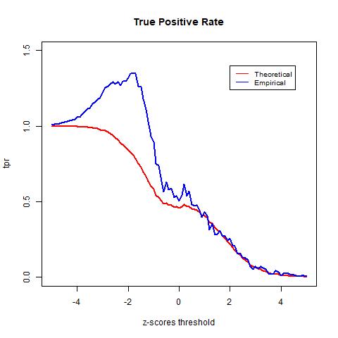
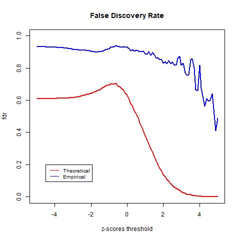
The TPR indicates the likelihood that an actual positive sample produces a positive testing result. In the graph above we see that the TPR of the empirical null goes above 1. This is due to mismatch between the data and the distribution, as observed in the previous histogram of the z-scores, the empirical null distribution goes above the histogram from around -4 to -2. The FPR indicates the likelihood of false positives. Lastly, we see that the theoretical null distribution yields a FDR curve that converges to 0 as the threshold x increases. Meanwhile, the empirical null distribution produces a much higher level FDR than the theoretical null distribution given the same level of threshold. Moreover, the FDR curve yielded by the empirical null distribution fails to converge as x increases and is approximately 0.44 when the threshold is the largest at x = 5. At first this may seem to be indications that the theoretical null outperforms the empirical null; however, this is not necessarily true. Since we do not have the actual labels of the data and instead only have an estimation of the error rate, we cannot know for sure the accuracy of either model. However, we know that the empirical null distribution adjusts for unknown factors empirically, it is likely to provide more realistic estimations and therefore more accurate results.

Discussion

The graph above shows that the theoretical null distribution yields a FDR curve that converges to 0 as the threshold x increases. Meanwhile, the empirical null distribution produces a much higher level FDR than the theoretical null distribution given the same level of threshold. Moreover, the FDR curve yielded by the empirical null distribution fails to converge as x increases and is approximately 0.44 when the threshold is the largest at x = 5.

At first, the above result seems to conflict with our hypothesis that the empirical null distribution will produce better results than the theoretical null distribution. While our result shows that the theoretical null distribution yields a lower FDR at the same level of threshold than the empirical null distribution, this does not necessarily mean that the theoretical null provides a more accurate result. Since we cannot know the actual label of the data, there is no way for us to actually test the accuracy of our result. What we have is an estimation of the error rate, which allows us to gain insight into the likelihood of false positives at each level of the threshold. The theoretical null distribution yields an apparent lower error rate, but this result may be incorrect. This is because that as we have observed, additional variance in the histogram, due to confounding factors, will skew the results of the theoretical null. In contrast, the empirical null distribution adjusts for those unknown confounding factors empirically. This results in lower detection power, as observed from the difference in the estimated parameter p₀, but the error rate may be more realistic, meaning it is closer to the true error rate.

References

Ahmed N, Yigit A, Isik Z, Alpkocak A. Identification of Leukemia Subtypes from Microscopic Images Using Convolutional Neural Network. Diagnostics. 2019; 9(3):104. https://doi.org/10.3390/diagnostics9030104

Efron, B., Tibshirani, R., Storey, J.D., Tusher, V., 2001. Empirical Bayes analysis of a microarray experiment. J. Am. Stat. Assoc. 96 (456), 1151-1160.

Golub TR, Slonim DK, Tamayo P, Huard C, Gaasenbeek M, Mesirov JP, Coller H, Loh ML, Downing JR, Caligiuri MA, Bloomfield CD, Lander ES. Molecular classification of cancer: class discovery and class prediction by gene expression monitoring. Science. 1999 Oct 15;286(5439):531-7. doi: 10.1126/science.286.5439.531. PMID: 10521349.

Schwartzman,A., Dougherty, R., Lee, J., Ghahremani, D., & Taylor, J. (2009). Empirical null and false discovery rate analysis in neuroimaging. NeuroImage, 44(1), 71–82.

“Types of Leukemia: Children’s Hospital Pittsburgh.” Children’s Hospital of Pittsburgh, www.chp.edu/our-services/cancer/conditions/leukemia/types.